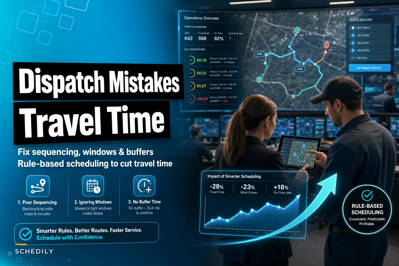

Field service dispatch optimization sounds like one of those problems you throw software at and hope for the best. But after watching hundreds of service businesses wrestle with the same patterns, the core issue is usually pretty clear: most dispatchers are working with scheduling rules that guarantee wasted windshield time before the day even starts.
The frustrating part? These aren't complex algorithmic failures. They're basic math errors that compound throughout the day. A plumbing company in Phoenix found their techs were averaging 2.8 hours of daily drive time for jobs that should have required 1.5 hours max. The problem wasn't traffic or poor routing — it was three specific dispatch rules that looked reasonable on paper but created cascading inefficiencies in practice.
Mistake #1: Using fixed 2-hour windows for everything
Walk into most HVAC dispatch offices and you'll see the same thing on their scheduling board: 8-10am, 10-12pm, 12-2pm, 2-4pm, 4-6pm. Clean blocks that make scheduling feel organized. Except this rigid structure forces techs to zigzag across service areas because the windows don't match actual job requirements.
A furnace inspection takes 45 minutes. A full system replacement takes 4-6 hours. Both get squeezed into the same fixed-window system, which creates two problems at once. Short jobs leave techs with dead time they can't fill because the next window hasn't started. Long jobs blow through multiple windows and trigger a domino effect of delays for the rest of the day.
The real damage happens in the gaps. When a tech finishes a 45-minute inspection at 9:15am, they can't start the 10am appointment early — so they sit in a parking lot or drive back toward the shop only to turn around again. Meanwhile, the 4-hour installation that kicked off at 8am is now bleeding into the noon slot, and dispatch is scrambling to reroute other techs.
The windowing policy that actually works
Quick jobs (under 60 minutes):
-
Dense areas
90-minute windows
-
Suburban
2-hour windows
-
Rural
3-hour windows
Standard jobs (1-3 hours):
-
Morning slots
arrival window only (8-10am arrival)
-
Afternoon slots
3-hour completion window
Major jobs (3+ hours):
-
First appointment only
-
Block the full estimated time plus 20% buffer
-
No windows, just "starting at X time"
A pest control company that switched to this approach cut daily drive time from 3.2 hours to 2.1 hours per tech. The improvement didn't come from better routing software — it came from eliminating the artificial constraints that were forcing inefficient routes from the start.
Mistake #2: Adding the same buffer time to every job type
Buffers exist for good reason — one bad job shouldn't detonate the rest of the schedule. So dispatchers add 30 minutes to everything. Feels safe. Except uniform buffers create almost as many problems as they prevent.
Eliminate scheduling conflicts and missed meetings.
Schedily helps you organize and manage all appointments and team availability effortlessly.
- Unified appointment and resource management
- Automated notifications & reminders
- Team calendar synchronization
No credit card required
Quick maintenance checks don't need 30-minute buffers. They need 10-15 minutes. Complex diagnostics might need 45-60. When you apply the same cushion across the board, you either waste capacity on simple jobs or set up complex ones to fail.
The math compounds fast. A tech doing six standard maintenance visits a day with 30-minute buffers is carrying three hours of unnecessary padding — enough time for two more service calls. Meanwhile, the tech handling complex repairs with that same 30-minute buffer is chronically late because diagnostic jobs routinely run 40-60% over estimate.
Buffer calculation based on variance, not averages
Tracking actual variance by job type is what separates decent dispatch from good dispatch. The formula:
Buffer Time = (90th percentile duration - median duration) × 0.75
Track job-duration variance weekly to catch shifting patterns before they force buffer changes.
Real example from an appliance repair company:
| Job Type | Median Time | 90th Percentile | Calculated Buffer |
|---|---|---|---|
| Diagnostic | 45 min | 75 min | 23 min |
| Standard Repair | 90 min | 120 min | 23 min |
| Part Replacement | 30 min | 40 min | 8 min |
| Complex Repair | 150 min | 210 min | 45 min |
Part replacements get minimal buffer because they're predictable. Complex repairs get substantial buffer because variance is high. That's not over-engineering — it's just acknowledging how these jobs actually behave in the field.
After switching from uniform 30-minute buffers to variance-based calculations, that same company went from completing 5.2 to 6.8 jobs per tech per day while actually reducing overtime hours.
Mistake #3: Sequencing jobs by proximity instead of SLA requirements
Every dispatcher knows the basic rule: cluster nearby jobs to minimize travel. Logical, efficient, and completely wrong when you factor in service level agreements.
Here's what plays out in practice. You've got four jobs in the same neighborhood — perfect for routing. So you stack them sequentially. Except one is a warranty repair with a 24-hour SLA expiring at 2pm. Another is a premium customer expecting morning service. The third has a 72-hour window. The fourth is an emergency that just came in.
By the time your tech arrives at the warranty job at 3:30pm, the SLA is blown, potentially triggering penalties or losing the service contract. The premium customer who expected morning service gets an afternoon visit. The flexible 72-hour call got done first because it happened to be the closest starting point.
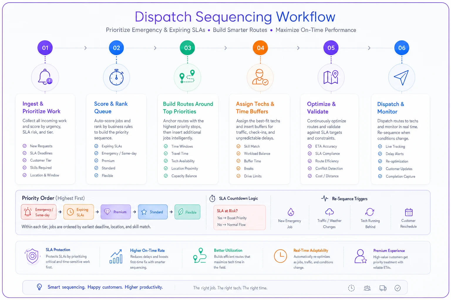
SLA-driven sequencing that preserves efficiency
The fix isn't abandoning geographic clustering — it's layering SLA priority on top of it. The sequencing hierarchy:
-
Emergency/Same-day SLAs (must complete today)
-
Expiring SLAs (less than 4 hours remaining)
-
Premium/Priority customers (even without strict SLA)
-
Standard SLAs (24-48 hour window)
-
Flexible scheduling (72+ hour window)
Within each tier, optimize for proximity. Between tiers, SLA requirements override travel efficiency.
In practice, this means starting each morning by identifying all jobs with SLAs expiring before 2pm. These become fixed stops regardless of location. Build routes around those critical appointments first, then fill in with geographically convenient standard calls.
This illustrates the sequencing flow used to prioritize SLAs before optimizing for distance.
A garage door repair company restructured dispatch around this hierarchy and eliminated SLA violations entirely — while only increasing average drive time by about 12 minutes per day. A small efficiency loss compared to avoiding $500 SLA penalties and keeping service contracts intact.
Sample schedule with real calculations
Here's how this plays out with actual numbers from a typical Tuesday — an HVAC company running four techs across a 30-mile service area.
Tech A - Commercial specialist:
-
7
30am: Drive to first job (15 miles, 25 min)
-
8
00am: Restaurant AC repair (SLA expires 10am, 120 min job + 45 min buffer)
-
10
45am: Drive to second job (8 miles, 15 min)
-
11
00am: Office building maintenance (90 min job + 23 min buffer)
-
1
00pm: Lunch break
-
2
00pm: Retail store diagnostic (Priority customer, 60 min + 23 min buffer)
-
3
30pm: Drive to final job (12 miles, 20 min)
-
3
50pm: Warehouse unit inspection (45 min + 8 min buffer)
-
4
45pm: Return to shop (18 miles, 30 min)
Total drive time: 110 minutes Total productive time: 315 minutes Efficiency: 74%
Tech B - Residential East:
-
8
00am: First appointment (5 miles from home, 10 min)
-
8
15am: Furnace diagnostic (45 min + 15 min buffer)
-
9
15am: Drive to cluster area (3 miles, 8 min)
-
9
25am: Three sequential maintenance calls (same neighborhood)
-
- House 1
30 min + 8 min buffer
-
- House 2
30 min + 8 min buffer
-
- House 3
45 min + 8 min buffer
-
12
00pm: Drive to afternoon area (11 miles, 18 min)
-
12
30pm: Lunch
-
1
30pm: Premium customer AC repair (90 min + 23 min buffer)
-
3
00pm: Final maintenance call (4 miles, 10 min drive, 30 min + 8 min buffer)
-
3
50pm: Return home (8 miles, 15 min)
Total drive time: 71 minutes Total productive time: 270 minutes Efficiency: 79%
Compare this to their old fixed-window system, where the same tech averaged 140 minutes of drive time for only four jobs per day. The density improvement came from clustering compatible jobs and using appropriate buffers — not from forcing everything into 2-hour blocks.
Why standard dispatch software keeps making these mistakes
Most field service platforms inherited their logic from package delivery routing, where every stop takes roughly the same amount of time and there's no customer interaction to manage. Those systems optimize for pure distance efficiency because that's what matters when you're dropping off boxes.
Service dispatch operates under completely different constraints. Job duration varies wildly. Customer availability matters. SLAs create hard deadlines. Equipment and parts affect sequencing. Yet most software still approaches it like a traveling salesman problem.
The result is dispatchers constantly overriding the system, which defeats the whole point. Or worse, they trust it — and then wonder why techs are always running late despite "optimized" routes.
This is actually an area where AI-powered operational platforms help in a meaningful way. Modern tools can track real job variance, calculate appropriate buffers automatically, and balance SLA requirements against travel efficiency without someone having to manually rebuild the logic every day. Instead of rigid rules, the system learns your patterns — which techs run fast or slow, which job types commonly extend, which customers are flexible versus strict about their windows.
An electrical contractor that switched from manual dispatch with fixed rules to an AI-assisted platform saw daily completed jobs jump from 5.8 to 7.2 per tech. Not because the system found magical routes, but because it stopped reinforcing the same systematic inefficiencies built into the old rule structure.
The buffer calculation template you can steal
Stop guessing at buffer times. Here's the exact template:
Step 1: Track actual durations for 30 days
-
Record estimated time
-
Record actual completion time
-
Note job type and complexity factors
Step 2: Calculate variance by job type
-
Find median duration (half above, half below)
-
Find 90th percentile (90% complete within this time)
-
Calculate spread
90th percentile minus median
Step 3: Apply the buffer formula
-
Standard jobs
Spread × 0.75
-
High-variance jobs
Spread × 1.0
-
Predictable jobs
Spread × 0.5
Step 4: Round to practical increments
-
Round up to nearest 5 minutes for scheduling simplicity
-
Never less than 10 minutes (minimum transition time)
-
Cap at 60 minutes (anything longer needs its own window)
Step 5: Review and adjust monthly
-
Track SLA violations and their root cause
-
Track idle time between appointments
-
Adjust buffers up if violations exceed 5%
-
Adjust buffers down if idle time exceeds 20%
Appliance repair companies using this template report around 22% improvement in daily job completion without increasing overtime.
Why everyone defaults to bad dispatch rules anyway
The fixed-window, uniform-buffer, proximity-first approach feels right because it's simple. Customers understand "we'll be there between 2 and 4." Dispatchers can quickly slot jobs into preset blocks. Techs know the rhythm.
But operational simplicity that creates inefficiency isn't actually simple — it's expensive. Those clean 2-hour windows force unnecessary miles. The uniform buffers waste capacity on routine jobs while setting up complex jobs to fail. The proximity-first routing saves 10 minutes of drive time while costing $500 in SLA penalties.
The resistance to variable scheduling usually comes from fear of added complexity. Different window sizes to manage, customers who might get confused by non-standard slots, a messier scheduling board.
Those concerns tend to fade fast once teams see the results. Techs would rather finish more jobs with less stress than sit in parking lots between fixed windows. Customers care more about showing up when expected than about symmetrical time slots. Dispatchers adapt quickly when SLA violations drop and capacity goes up.
Your next step: Run the diagnostic
Before changing anything, get your baseline. For the next five days, track:
-
Actual drive time per tech per day
-
Number of SLA violations and their root cause
-
Idle time between appointments
-
Jobs that exceeded their scheduled window
-
Jobs rescheduled due to cascading delays
Most operations find they're losing 25-35% of field capacity to bad dispatch rules. That number is usually enough to motivate action.
Then pick one mistake to fix first — whichever one is causing the most immediate pain. Getting daily SLA violations? Start with sequencing. Techs drowning in windshield time? Fix the window policy. Delays cascading through the whole day? Address buffers first.
The compound effect happens faster than most expect. Better windows reduce travel time. Appropriate buffers prevent cascading delays. SLA-based sequencing eliminates penalties. Together, they turn dispatch from daily firefighting into something that actually runs predictably.
The businesses that get field service dispatch right aren't all running complex algorithms or expensive software — though good tools definitely help. They're using basic scheduling rules that match operational reality instead of forcing reality to fit convenient blocks on a board.
Your techs already know these problems exist. They've complained about the 2-hour window for 30-minute jobs since day one. They've flagged the SLA violations coming from bad sequencing. They've sat in those parking lots burning fuel and scrolling their phones.
The math is straightforward. The rules are proven. The only thing standing between current chaos and efficient dispatch is deciding to stop accepting "that's how we've always done it" as an operational strategy.
Ready to optimize your scheduling and operations?
Join thousands of businesses using Schedily to save time, improve coordination, and enhance operational efficiency.