


Every appointment-based business faces the same operational nightmare: Monday morning you're overstaffed with technicians scrolling their phones, Thursday afternoon customers are walking out because wait times hit 90 minutes. The worst part? This pattern repeats every single month, yet most businesses still schedule based on gut feel or whatever worked last year.
The same gap keeps showing up across businesses ranging from 8-person veterinary clinics to 200-employee home service companies. They drown in appointment data but never translate it into actual staffing decisions. They track bookings, completions, cancellations — then completely ignore all of it when building next month's schedule.
That gap costs real money. A regional HVAC company was burning roughly $14,000 monthly on unnecessary overtime during shoulder season because they never adjusted baseline staffing after summer ended. A medical testing lab was losing around $22,000 in potential revenue each quarter by understaffing evening slots — the demand was there, they just kept scheduling like it was 2019.
Why appointment patterns don't automatically translate to staffing needs
The disconnect happens because appointment demand and workforce capacity operate on completely different time scales. Your appointment system shows Sally booked for 2pm next Tuesday. Your staffing system needs to know whether you need 3 or 4 technicians working that shift. Those aren't the same question.
Most businesses try to bridge this with basic math: "We average 40 appointments daily, each takes 30 minutes, so we need 20 work hours, which means 3 full-time staff." This falls apart almost immediately in real operations.
Appointment distribution never follows neat patterns. A dental office might see 70% of weekly appointments clustered between Tuesday and Thursday, 10am to 2pm — yet staff Monday through Friday equally, creating waste on slow days and bottlenecks during rush periods.
Appointment types also require completely different resource allocations. A quick oil change needs one tech for 20 minutes. A transmission diagnostic might need two techs for 90 minutes plus specialized equipment. Treating these as equivalent "appointments" in your forecast guarantees mismatches.
Then seasonal patterns layer in more complexity. The tax prep office that needs 12 preparers in March but only 3 in July. The pet grooming salon where December demand triples but only for specific services. These patterns hide in your appointment history — standard scheduling approaches miss them entirely.
Building demand curves from actual appointment data
The path from appointment chaos to predictable staffing starts with demand curves — representations of when work actually happens in your business. Not when appointments are booked, not when customers prefer, but when work gets done.
Eliminate scheduling conflicts and missed meetings.
Schedily helps you organize and manage all appointments and team availability effortlessly.
- Unified appointment and resource management
- Automated notifications & reminders
- Team calendar synchronization
No credit card required
Start by pulling appointment completion data for the past 12 months. You want completion timestamps, service types, actual duration (not scheduled duration), and resource requirements. That's the raw material for pattern recognition.
Step 1: Normalize your appointment types
Group services into operational categories based on resource needs, not marketing names. An auto repair shop might look like this:
Category A — Quick Services (single tech, under 30 min)
-
Oil changes
-
Tire rotations
-
Battery tests
-
Wiper replacements
Category B — Diagnostic Work (single tech, 30–90 min)
-
Check engine light diagnosis
-
Brake inspections
-
Alignment checks
-
AC system tests
Category C — Major Repairs (multiple techs/bays, 2+ hours)
-
Engine work
-
Transmission service
-
Suspension overhauls
-
Electrical system repairs
Each category has distinct workforce implications. Twenty Category A appointments might need 2 techs. Twenty Category C appointments might need 6 techs plus your senior diagnostic specialist.
Step 2: Map temporal distribution patterns
Plot your normalized appointments across three time dimensions: hour of day, day of week, week of month. This is where the real patterns emerge.
Here's what this looked like for a mobile pet grooming business:
| Time Period | Mon | Tue | Wed | Thu | Fri | Sat | Sun |
|---|---|---|---|---|---|---|---|
| 8am–10am | 12% | 8% | 7% | 9% | 14% | 22% | 3% |
| 10am–12pm | 18% | 14% | 13% | 15% | 19% | 28% | 5% |
| 12pm–2pm | 8% | 11% | 10% | 12% | 11% | 15% | 4% |
| 2pm–4pm | 14% | 16% | 15% | 17% | 16% | 18% | 6% |
| 4pm–6pm | 9% | 12% | 13% | 14% | 10% | 8% | 2% |
That Saturday morning surge jumps off the page — nearly 50% of Saturday appointments cluster before noon. Yet they were scheduling groomers evenly throughout Saturday, creating morning chaos and afternoon waste.
Step 3: Layer in seasonal variations
Monthly patterns matter just as much as daily ones. Pull monthly appointment totals and calculate variance from your annual average.
-
March–April
70% of average (startup season)
-
May–August
140% of average (peak season)
-
September–October
95% of average (maintenance mode)
-
November–February
45% of average (minimal service)
These aren't minor fluctuations. Peak season needs roughly triple the workforce of winter months. Miss this and you're either burning cash on idle workers or losing revenue to unmet demand.
Here's a simple workflow for building demand curves from appointment data.
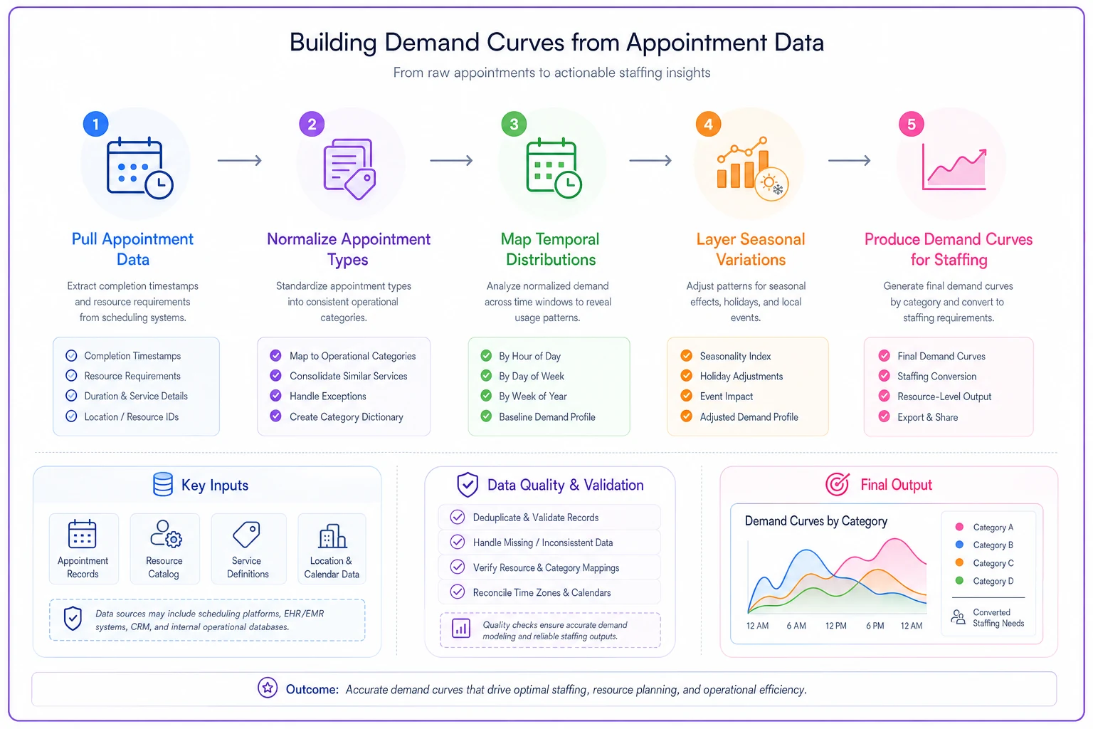
The diagram shows each step and the key data inputs.
Converting demand curves into headcount requirements
Raw demand curves tell you when work happens. Converting them into actual headcount needs requires understanding your operational constraints and efficiency factors.
The basic conversion formula
Required Headcount = (Total Work Minutes / Available Minutes per Worker) × Efficiency Factor
Simple enough, but each component hides real complexity.
Total Work Minutes includes:
-
Direct appointment time
-
Prep and cleanup time
-
Documentation requirements
-
Travel time between appointments (for mobile services)
-
Required breaks and administrative tasks
Available Minutes per Worker accounts for:
-
Scheduled shift length
-
Mandatory breaks
-
Typical bathroom and water breaks
-
Shift handoff time
-
Peak performance windows (workers aren't equally productive across 8 hours)
Efficiency Factor captures:
-
New employee learning curves
-
Complexity variations within service categories
-
Customer-induced delays
-
Equipment availability constraints
A realistic example from an automotive quick-lube shop:
-
Average oil change
20 minutes direct service
-
Add 5 minutes for vehicle positioning and customer interaction
-
Add 3 minutes for point-of-sale and documentation
-
Total per appointment
28 minutes
During a typical Saturday 8am–12pm shift:
-
240 total minutes per worker
-
Minus 15 minutes for break
-
Minus 10 minutes for setup/cleanup
-
Available productive time
215 minutes
At 85% efficiency (accounting for variations and delays), each worker handles about 183 productive minutes — roughly 6.5 oil changes per worker per 4-hour shift.
If Saturday morning demand averages 26 oil changes, you need 4 workers scheduled.
Accounting for service mix complexity
Real operations rarely involve single service types. Your demand curves need to reflect the resource intensity of different appointment categories.
Create a weighted demand score:
| Service Category | Avg Duration | Complexity Weight | Resource Multiplier |
|---|---|---|---|
| Category A | 30 min | 1.0 | 1 worker |
| Category B | 75 min | 1.8 | 1 worker |
| Category C | 150 min | 3.2 | 2 workers |
A physiotherapy clinic tracked their Wednesday afternoons:
-
6 initial assessments (Category C)
6 × 3.2 = 19.2 weighted units
-
12 follow-up treatments (Category B)
12 × 1.8 = 21.6 weighted units
-
8 quick adjustments (Category A)
8 × 1.0 = 8.0 weighted units
Total weighted demand: 48.8 units. If each therapist handles 12 weighted units per 4-hour shift, you need 4.1 therapists — round up to 5 for that window.
Creating shift templates that match demand reality
Standard shift templates — 9-to-5, Monday through Friday — almost never align with actual appointment demand. Building templates around your demand curves reduces both labor costs and service delays.
Core principles for shift design
Principle 1: Peak coverage without baseline bloat
Instead of staffing for peaks all day, create overlapping shifts that concentrate coverage when it's needed.
-
1 vet
7am–3pm (handles morning drop-offs)
-
2 vets
10am–6pm (peak appointment hours)
-
1 vet
12pm–8pm (afternoon surgeries and emergencies)
This provided 4 vets during the 12pm–3pm rush while cutting total labor hours by about 20%.
Principle 2: Variable shift lengths match demand duration
Not every peak needs 8-hour coverage. A restaurant equipment repair company noticed emergency calls clustering 11am–2pm (lunch rush issues) and 5pm–8pm (dinner rush problems).
-
3-hour "lunch response" shifts (11am–2pm)
-
4-hour "dinner response" shifts (4pm–8pm)
-
Traditional full shifts for baseline coverage
Part-time workers loved the flexibility. The company reduced overtime by around 60%.
Principle 3: Skills-based scheduling for complex services
When appointment types require specific expertise, generic headcount planning falls apart. Map demand curves by skill requirement.
-
Maintenance calls (any certified tech)
-
Installation work (installation specialist required)
-
Diagnostic calls (senior tech required)
-
Emergency repairs (on-call senior tech)
Their Thursday shift template became:
-
2 maintenance techs
8am–4pm
-
1 installation specialist
7am–3pm
-
1 senior diagnostic tech
10am–6pm
-
1 flex tech
12pm–8pm (handles overflow and emergencies)
Practical shift template examples
Medical Testing Lab Pattern:
Monday–Wednesday (steady flow):
-
Shift A
6am–2pm (2 techs)
-
Shift B
8am–4pm (3 techs)
-
Shift C
12pm–8pm (2 techs)
-
Shift D
2pm–10pm (1 tech)
Thursday–Friday (insurance deadline rush):
-
Shift A
6am–2pm (3 techs)
-
Shift B
8am–4pm (5 techs)
-
Shift C
10am–6pm (4 techs)
-
Shift D
12pm–8pm (3 techs)
-
Shift E
2pm–10pm (2 techs)
Saturday (walk-in focused):
-
Morning burst
7am–11am (4 techs)
-
Midday coverage
10am–2pm (3 techs)
-
Afternoon wind-down
1pm–5pm (2 techs)
Home Service Company Pattern:
During summer AC season:
-
Dawn patrol
6am–2pm (2 techs, handle emergencies from overnight)
-
Morning wave
8am–4pm (6 techs, primary appointment block)
-
Afternoon coverage
12pm–8pm (4 techs, afternoon appointments plus callbacks)
-
Evening emergencies
4pm–12am (2 techs, emergency calls only)
During winter heating season, the pattern inverts — fewer dawn patrol shifts, heavier evening coverage, expanded weekends because people are home to notice heating problems.
The forecast-to-hiring calculator framework
Converting forecasted demand into hiring decisions requires more than simple math. You need a systematic approach that accounts for employee turnover, training time, and seasonal variations.
Building your baseline model
Start with your core demand converted to FTE (Full-Time Equivalent) requirements:
-
Calculate average weekly appointment demand by category
-
Apply your conversion formula for headcount needs
-
Sum across all time periods for total hours needed
-
Divide by standard full-time hours (usually 40) for FTE count
A dental practice example:
-
Weekly weighted demand
850 units
-
Conversion rate
12 units per hygienist per day
-
Daily hygienist days needed
71
-
Weekly requirement
14.2 hygienist work days
-
FTE requirement
14.2 / 5 = 2.84 FTE
But 2.84 FTE doesn't mean hire 3 full-time hygienists.
Adjusting for operational realities
Turnover buffer: Industry turnover rates directly affect hiring needs. If hygienist turnover averages 20% annually, you need 3.41 FTE positions filled to maintain 2.84 FTE production.
Training runway: New employees don't hit full productivity immediately. A mobile phone repair shop tracked new technician productivity:
-
Week 1–2
30% productivity
-
Week 3–4
60% productivity
-
Week 5–8
85% productivity
-
Week 9+
100% productivity
Factor this ramp-up into your hiring timeline. If you need additional capacity in June, start hiring in March.
Seasonal flex calculations: For businesses with significant seasonal swings, maintain a core team plus flex capacity:
-
Core team = Minimum season demand × 1.1 (small buffer)
-
Flex needs = Peak season demand − Core capacity
A landscaping company might need:
-
Core team
4 FTE (handles winter minimum plus 10%)
-
Summer flex
+8 FTE (temporary or seasonal workers)
-
Spring/Fall flex
+3 FTE (part-time or contractors)
The simple calculator template
Build a spreadsheet with these inputs:
Demand Inputs:
-
Appointments per week by category
-
Average duration per category
-
Complexity weighting per category
-
Seasonal adjustment factors
Operational Inputs:
-
Standard shift lengths
-
Efficiency factors by experience level
-
Training productivity curves
-
Expected turnover rates
Calculate:
-
Weighted weekly demand = Sum(Appointments × Duration × Complexity)
-
Base FTE needed = Weighted demand / (Weekly hours × Efficiency)
-
Turnover-adjusted FTE = Base FTE / (1 − Turnover Rate)
-
Hiring needs = Turnover-adjusted FTE − Current Staff + Growth Factor
Output:
-
FTE requirements by month
-
Hiring timeline with training buffers
-
Shift templates by day/season
-
Part-time vs full-time mix recommendations
Running this monthly keeps your forecast current rather than relying on a number you calculated once in January and never revisited.
Common forecasting mistakes that break workforce planning
Even with solid frameworks, certain mistakes consistently derail appointment-based workforce forecasting.
Mistake 1: Using booking patterns instead of completion patterns
Customers book appointments based on their preference. Work happens based on your operations. These rarely line up perfectly.
A massage therapy clinic found that customers booked Thursday appointments two weeks in advance but Saturday appointments only three days ahead. Planning staff based on advance bookings meant overstaffing Thursdays and scrambling for Saturday coverage.
Track when work actually happens, not when customers decide they want it.
Mistake 2: Ignoring appointment interdependencies
Some appointments create cascade effects on resources. An orthodontist practice learned this the hard way — emergency repair appointments (broken brackets) took 15 minutes but disrupted the next two or three scheduled appointments, effectively consuming 45–60 minutes of productivity.
-
Emergency slots that can't be pre-booked
-
Overflow providers for schedule recovery
-
Clear escalation rules for delays
Build buffers around high-disruption appointment types:
Mistake 3: Forecasting at the wrong granularity
Company-wide forecasts miss location-specific patterns. Location-specific forecasts can miss service-line variations. A multi-location urgent care group initially forecasted at the company level, showing steady demand. Location-level analysis revealed something completely different:
-
Downtown location
70% of visits during weekday lunch hours
-
Suburban location
Evening and weekend concentration
-
University location
Massive swings based on academic calendar
Each location needed a completely different staffing model despite similar overall volume.
Mistake 4: Not accounting for forecast uncertainty
Your demand forecast is a prediction, not a guarantee. Build uncertainty ranges into your planning:
| Scenario | Demand Variance | Staffing Response |
|---|---|---|
| Best case | +20% above forecast | Activate on-call/part-time pool |
| Expected case | Core forecast | Staff at base headcount |
| Worst case | −20% below forecast | Reduce flex shifts first |
In practice this usually means keeping core staff at around 85% of expected demand, maintaining an on-call or part-time pool for surge situations, and cross-training so workers can flex between roles when needed.
Software automation for forecast-to-schedule workflows
Getting from demand curves to an actual posted schedule involves dozens of intermediate steps. Manual processes here virtually guarantee errors — mismatched skills, double-bookings, coverage gaps that nobody catches until a customer complains.
Modern appointment-based businesses need operational software that connects forecasting to scheduling. Not something that promises to predict everything automatically, but practical automation that handles repetitive conversion work while keeping human judgment in the loop for exceptions.
The most valuable automations focus on data flow and constraint checking. Your appointment system already knows next month's bookings. Your HR system knows who's available, their skills, and their scheduled time off. Operational software bridges these systems, surfacing conflicts before they become service failures — not after customers start complaining about delays.
When seasonal patterns suggest ramping up staff, the platform can trigger hiring workflows with appropriate lead times built in. When demand for certified technicians exceeds available certified staff on a particular shift, that gets flagged immediately rather than discovered at 9am when the team shows up short.
A small medical practice that spent six hours weekly manually building schedules now spends about 30 minutes reviewing and adjusting system recommendations. That's 5+ hours redirected toward actually running the business — not spreadsheet archaeology.
Moving from reactive scrambling to predictive workforce planning
Businesses that successfully implement appointment-based workforce forecasting share a few common traits. They stop treating scheduling as a weekly firefight and start viewing it as a predictable operational process.
They commit to data discipline. Every appointment gets properly categorized. Actual service times get tracked, not just scheduled durations. When patterns shift, they investigate why rather than just adjusting on the fly.
They also accept that perfect forecasts don't exist — but good-enough forecasts beat pure guesswork every time. A home inspection company improved their staffing match rate from around 60% to 85% just by implementing basic demand curves and shift templates. Not perfect, but the reduction in overtime costs and customer complaints transformed their operations.
Third, they build flexibility into their workforce structure. Instead of trying to staff precisely for predicted demand, they maintain core coverage with systematic flex capacity. Part-time pools, cross-trained employees, and partnership agreements with staffing agencies provide surge capacity without bloating baseline costs.
The path from appointment chaos to workforce predictability isn't complicated, but it does require systematic thinking and consistent execution. Start with your appointment history. Build your demand curves. Create shift templates that match reality. Then iterate based on actual results rather than hoping next month will somehow be different.
Your appointments already tell you what's coming. The question is whether you'll actually use that data or keep scheduling based on last year's guess.
Ready to optimize your scheduling and operations?
Join thousands of businesses using Schedily to save time, improve coordination, and enhance operational efficiency.